This page documents the passages required to extract PhenoRice results for the different polygons of the RiceAtlas dataset. Input data are the raster mosaics stored in Data/orig_mosaics, and the reshuffled riceAtlas shapefile stored in Data/vector/Ricetlas/riceatlas_asia_reshuffled.shp

Extract data for a specific RiceAtlas region

Suppose you want to extract data for Region: “Region_3_-_Central_Luzon“:

#   ____________________________________________________________________________
#   set input and output folders                                            ####

# set the main folder ----
main_folder <- "/home/lb/my_data/prasia/Data"

#'  # Suppose you want to extract data for Region: "Region_3_-_Central_Luzon" :
#'  # --> extract it from the full shapefile

Region_name <- "Region_3_-_Central_Luzon"

## "1) run "pr_extract" on the region ----

pr_extract(main_folder,
           region = Region_name)

NOTE: Using region = "All" will automatically process all RiceAtlas regions.

The function crops the original mosaics on the selected region, and then extracts the data for the different sub-regions of the specified RiceAtlas regions.

Cropped rasters are stored in the Data/subsets/_region_name_/orig and Data/subsets/_region_name_/decirc folders.
Extracted data are saved in the Data/subsets/_region_name_/RData folder. One separate RData file is created for each PhenoRice parameter (e.g., “Dhaka_sos_stats.RData”, “Dhaka_eos_stats.RData”, “Dhaka_sos_decirc_stats.RData”)

Accessing the extracted data

Extracted data can be successively accessed by loading the saved RData files. Here I show it for the “sos” dataset of “Central_luzon”.

main_folder <- "/home/lb/my_data/prasia/Data"
indata <- get(load(file.path(main_folder,
                             "subsets/Region_3_-_Central_Luzon/RData/Region_3_-_Central_Luzon_sos_stats.RData")))

The data is saved as a list containing two elements:

indata$alldata contains “raw” info extracted from all pixels of the selected region that were recognized as “rice” in the different years:

head(indata$alldata)

## # A tibble: 6 x 8
##                                 ID_name variable band_n  year       date   doy     N n_pix_val
##                                  <fctr>    <chr>  <int> <dbl>     <date> <dbl> <int>     <int>
## 1 PHL_Region 3 - Central Luzon_Zambales      sos      1  2003 2002-10-25   -68     1        33
## 2 PHL_Region 3 - Central Luzon_Zambales      sos      1  2003 2002-08-30  -124     2        33
## 3 PHL_Region 3 - Central Luzon_Zambales      sos      1  2003 2002-09-15  -108     3        33
## 4 PHL_Region 3 - Central Luzon_Zambales      sos      1  2003 2002-08-22  -132     4        33
## 5 PHL_Region 3 - Central Luzon_Zambales      sos      1  2003 2002-10-01   -92     5        33
## 6 PHL_Region 3 - Central Luzon_Zambales      sos      1  2003 2002-10-01   -92     6        33

It contains the following columns:

ID_name : Name of RiceAtlas polygon
variable : PhenoRice variable
band_n : band of the tiff mosaics from which values come from (e.g., 1 = 2003 seas. 1; 2 = 2003 seas 2….)
year : year of the analysis (note that “date” can correspond to a different year on seasons spanning end of the yea (e.g., year = 2003, sos date = 2002-10-25)
date : date of occurrence of the PhenoRice metric
doy : doy of occurrence of the PhenoRice metric (for the “decirc” variables this is the number of days since 2000-01-01; for “standard” varibales, it is number of days since the beginning of the year (negative values possible as well as values above 365!))
N : unique identifier of a pixel within the subregion
n_pix_val: number of pixels identified as being rice within the subregion

so, for example, subsetting on a specific “ID_NAME” gives us all PhenoRice results for a given subregion:

require(dplyr)
pix_data <- indata$alldata %>% 
  dplyr::filter(ID_name == "PHL_Region 3 - Central Luzon_Zambales")
head(pix_data)

## # A tibble: 6 x 8
##                                 ID_name variable band_n  year       date   doy     N n_pix_val
##                                  <fctr>    <chr>  <int> <dbl>     <date> <dbl> <int>     <int>
## 1 PHL_Region 3 - Central Luzon_Zambales      sos      1  2003 2002-10-25   -68     1        33
## 2 PHL_Region 3 - Central Luzon_Zambales      sos      1  2003 2002-08-30  -124     2        33
## 3 PHL_Region 3 - Central Luzon_Zambales      sos      1  2003 2002-09-15  -108     3        33
## 4 PHL_Region 3 - Central Luzon_Zambales      sos      1  2003 2002-08-22  -132     4        33
## 5 PHL_Region 3 - Central Luzon_Zambales      sos      1  2003 2002-10-01   -92     5        33
## 6 PHL_Region 3 - Central Luzon_Zambales      sos      1  2003 2002-10-01   -92     6        33

from which we will be able to extract all kind of information without bothering anymore with the homungus raster mosaics! For example:

library(ggplot2)
ggplot(pix_data) + geom_violin(aes(x = factor(year), y = doy), alpha = 0.4) + 
  theme_bw() + 
  ggtitle("Sos Dates distribution - Central Luzon_Zambales") + 
  coord_flip()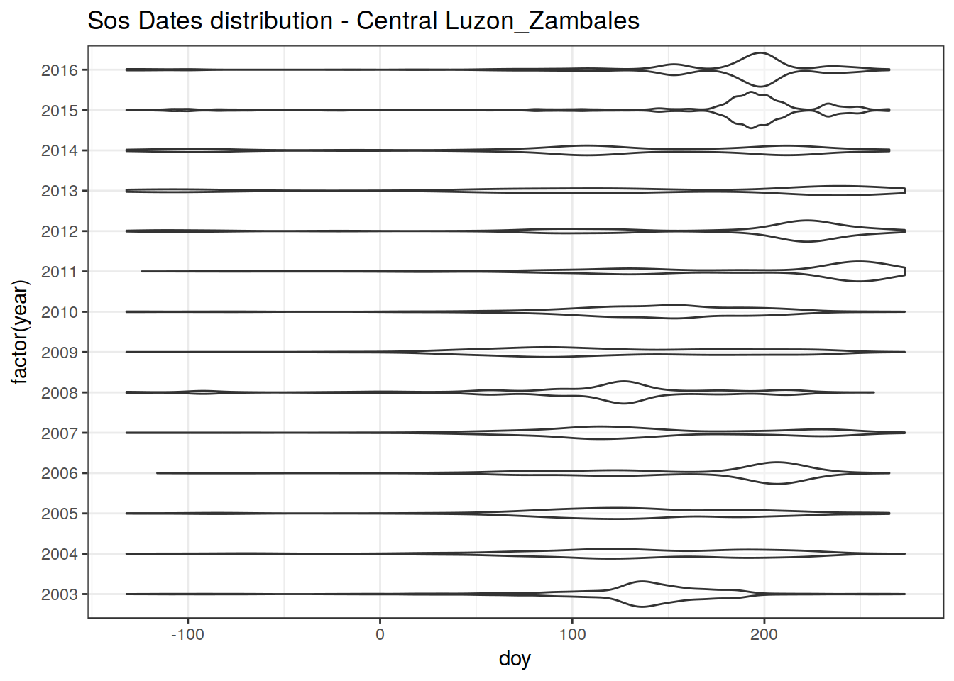

indata$stats contains “summarized” data over each subregion and PhenoRIce season:

head(indata$stats)

## # A tibble: 6 x 12
##                                 ID_name variable band_n  year    avgdate    avgdoy meddoy       sd mindoy maxdoy n_pix_val n_pix
##                                  <fctr>    <chr>  <dbl> <dbl>     <date>     <dbl>  <dbl>    <dbl>  <dbl>  <dbl>     <int> <int>
## 1 PHL_Region 3 - Central Luzon_Zambales      sos      1  2003 2002-09-28 -94.18182    -92 18.89685   -132    -60        33 68393
## 2 PHL_Region 3 - Central Luzon_Zambales      sos      2  2003 2003-02-02  32.98810     33 29.54698    -28     81        84 68393
## 3 PHL_Region 3 - Central Luzon_Zambales      sos      3  2003 2003-05-07 126.77627    129 28.05247     17    177       885 68393
## 4 PHL_Region 3 - Central Luzon_Zambales      sos      4  2003 2003-06-08 158.70012    153 27.79479    105    273       807 68393
## 5 PHL_Region 3 - Central Luzon_Zambales      sos      5  2004 2003-10-10 -82.85714    -72 22.02431   -132    -60        56 68393
## 6 PHL_Region 3 - Central Luzon_Zambales      sos      6  2004 2004-01-31  30.27143     33 31.37844    -60     81        70 68393

ID_name : Name of RiceAtlas polygon
variable : PhenoRice variable
band_n : band of the tiff mosaics from which values come from (e.g., 1 = 2003 seas. 1; 2 = 2003 seas 2….)
year : year of the analysis (note that “date” can correspond to a different year on seasons spanning end of the yea (e.g., year = 2003, sos date = 2002-10-25)
avgdate : Average date of occurrence of the PhenoRice metric over the “band” and sub region
avgdoy : Average doy of occurrence of the PhenoRice metric over the “band” and sub region (the same conventions for decirc and original variables described above apply)
meddoy : Median doy of occurrence of the PhenoRice metric over the “band” and sub region
sd : Standard deviation of doy of occurrence of the PhenoRice metric over the “band” and sub region
mindoy : Minimum doy of occurrence of the PhenoRice metric over the “band” and sub region
maximum : Maximum doy of occurrence of the PhenoRice metric over the “band” and sub region
n_pix_val : number of pixels identified as being rice within the subregion
n_pix : total number of pixels within the subregion

(Note that for the current analysis this is not very useful, since the summaruized data are computed on a “per phenorice season” basis. It is better to use the “alldata” element of the output and perform any needed data extraction / summarization starting from that.)

Next steps

Preliminary analysis of consistency between PhenoRice and RiceAtlas

by comparing Phenorice histograms with riceatlas data. Histograms can be quickly produced like this:

library(sprawl)
# Create a dummy variable, aggregating all data as if they were from the same year
indata$alldata$fakedate <- sprawl::doytodate(indata$alldata$doy, 2003)

library(ggplot2)
ggplot(indata$alldata) +
  geom_histogram(aes(x = fakedate), binwidth = 8) +
  facet_wrap(~ID_name, scales = "free_y") + theme_bw()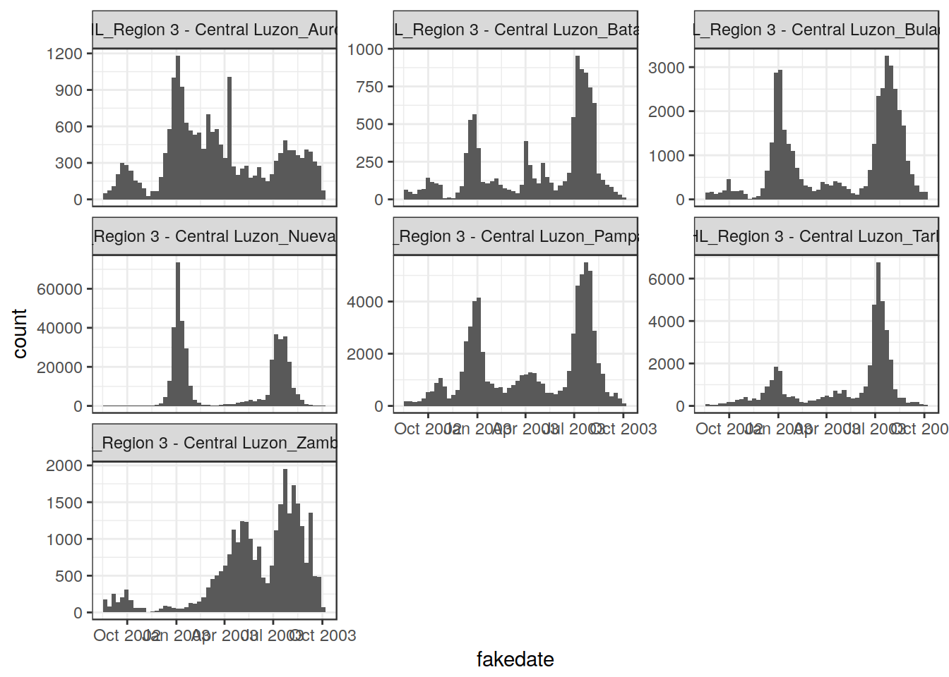

Info about the riceatlas season area and the sos ranges should be overplotted for reference to allow a quick comparison.

mixtools analysis to “identify” the main seasons

Needs to be done for each RiceAtlas polygon. We should decide if:

Subsetting the data on a selected year, and analyse only that one.
Analysing each year separately
Aggregating all data as if they were from the same year (this allows to increase the dimensions of the sample in low rice fc areas). This requires creating a “dummy variable” using something like:

indata$alldata$fakedate <- doytodate(datetodoy(indata$alldata$date), 2003)
head(indata$alldata)

## # A tibble: 6 x 9
##                                 ID_name variable band_n  year       date   doy     N n_pix_val   fakedate
##                                  <fctr>    <chr>  <int> <dbl>     <date> <dbl> <int>     <int>     <date>
## 1 PHL_Region 3 - Central Luzon_Zambales      sos      1  2003 2002-10-25   -68     1        33 2003-10-25
## 2 PHL_Region 3 - Central Luzon_Zambales      sos      1  2003 2002-08-30  -124     2        33 2003-08-30
## 3 PHL_Region 3 - Central Luzon_Zambales      sos      1  2003 2002-09-15  -108     3        33 2003-09-15
## 4 PHL_Region 3 - Central Luzon_Zambales      sos      1  2003 2002-08-22  -132     4        33 2003-08-22
## 5 PHL_Region 3 - Central Luzon_Zambales      sos      1  2003 2002-10-01   -92     5        33 2003-10-01
## 6 PHL_Region 3 - Central Luzon_Zambales      sos      1  2003 2002-10-01   -92     6        33 2003-10-01

Compute the PhenoRice Areas

Once the main seasons are identified, compute the area detected by PhenoRice within each season (by subsetting on date/fakedate)

Summarize the Comparison

Find a “statistical” way to compare both the detected rice seasons and areas and summarize results of the comparison.

Processing passages - Data Extraction Simplified