Extracting statistics for features of a vector file form a multi-band raster file
Source:vignettes/articles/extract_rast_example.Rmd
extract_rast_example.RmdCase Study
You have a raster multi-band file containing the values of an index (e.g., EVI) for multiple dates, and a vector file with areas from which you wish to either:
- Extract the time serie for each pixel contained in polygon ;
- Compute summary statistics on the values of the pixels of each polygon, for each date/band of the raster
Solution
You can use sprawl::extract_rast to quickly extract both the single-pixel time series, and the statistics for each polygon and date
Example
First of all, open the input raster containing the time series, and of the input vector file containing the polygons (i.e., the ROIs) for which you want the values.
# Here I'm using test datasets accessed on the filesystem, but on common usage it would as
# simple as `in_polys <- read_vect("D:/mypath/myfolder/lc_polys.shp"")

library(raster)
library(sprawl)


in_polys <- read_vect(system.file("extdata/shapes","lc_polys.shp",
                                  package = "sprawl.data"))
in_rast  <- stack(system.file("extdata/MODIS_test", "EVIts_test.tif",
                              package = "sprawl.data"))
Now, in in_polys we have a vector with 13 polygons:
## Simple feature collection with 13 features and 4 fields
## geometry type:  POLYGON
## dimension:      XY
## bbox:           xmin: 120.1778 ymin: 15.15353 xmax: 121.3394 ymax: 16.09343
## epsg (SRID):    4326
## proj4string:    +proj=longlat +datum=WGS84 +no_defs
## # A tibble: 13 x 5
##       id lc_type   category sup_catego                             geometry
##    <dbl> <chr>     <chr>    <chr>                             <POLYGON [°]>
##  1     1 forest_1  Forest   Vegetation ((120.7302 15.784, 120.7369 15.784,…
##  2     2 forest_2  Forest   Vegetation ((120.3664 15.39973, 120.3672 15.40…
##  3     3 urban_1   Other    Other      ((120.5941 15.49767, 120.5947 15.49…
##  4     4 cropland… Cropland Vegetation ((120.6371 15.46567, 120.6403 15.47…
##  5     5 cropland… Cropland Vegetation ((120.7231 15.54363, 120.7406 15.54…
##  6     6 forest_3  Forest   Vegetation ((121.2256 16.00655, 121.2387 16.01…
##  7     7 reiver_b… Other    Other      ((120.4208 15.33119, 120.4253 15.33…
##  8     8 cropland… Cropland Vegetation ((120.7702 15.36887, 120.7725 15.37…
##  9     9 urban_2_… Other    Other      ((120.5833 15.17092, 120.5999 15.17…
## 10    10 sparsfor… Forest   Vegetation ((120.1958 15.17424, 120.2063 15.17…
## 11    11 water     Other    Other      ((121.1377 15.85625, 121.1646 15.84…
## 12    12 small_fe… Other    Other      ((120.78 15.93824, 120.7811 15.9381…
## 13    13 out_feat  Other    Other      ((120.6781 16.09343, 120.6942 16.08…
, and in in_rast a raster time series with 46 bands:
## class : RasterStack
## dimensions : 447, 331, 147957, 46 (nrow, ncol, ncell, nlayers)
## resolution : 231.6564, 231.6564 (x, y)
## extent : 12897004, 12973683, 1685995, 1789545 (xmin, xmax, ymin, ymax)
## coord. ref. : +proj=sinu +lon_0=0 +x_0=0 +y_0=0 +a=6371007.181 +b=6371007.181 +units=m +no_defs
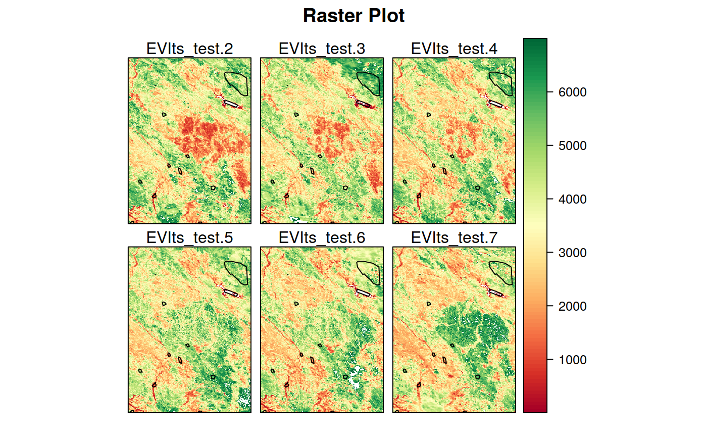
## names : EVIts_test.1, EVIts_test.2, EVIts_test.3, EVIts_test.4, EVIts_test.5, EVIts_test.6, EVIts_test.7, EVIts_test.8, EVIts_test.9, EVIts_test.10, EVIts_test.11, EVIts_test.12, EVIts_test.13, EVIts_test.14, EVIts_test.15, ...
## min values : -621, -813, -834, -559, -323, -680, -557, -1886, -861, -884, -917, -550, -540, -1948, -1912, ...
## max values : 9971, 9167, 9307, 9988, 8706, 9767, 9740, 9939, 8452, 9358, 9983, 8504, 9858, 9976, 9980, ...Let’s have a look at some bands:
To extract the values of pixels included in each polygon, you can then use simply:
extracted_values <- extract_rast(in_rast, in_polys)The output extracted values is a list containing two components:
-
extracted_values$alldatacontains the values for each extracted pixel, along with information extracted from the vector file. Additionally, the number of pixels extracted from each polygon is shown in theN_PIXcolumn, and an identifier to each pixel in theNcolumn
## Simple feature collection with 6 features and 9 fields
## geometry type:  POINT
## dimension:      XY
## bbox:           xmin: 12918200 ymin: 1754797 xmax: 12919360 ymax: 1754797
## epsg (SRID):    NA
## proj4string:    +proj=sinu +lon_0=0 +x_0=0 +y_0=0 +a=6371007.181 +b=6371007.181 +units=m +no_defs
## # A tibble: 6 x 10
##   lc_type band_n band_name n_pix_val     N value    id category sup_catego
##   <fct>    <int> <chr>         <int> <int> <dbl> <dbl> <fct>    <fct>
## 1 forest…      1 EVIts_te…        61     1  4454     1 Forest   Vegetation
## 2 forest…      1 EVIts_te…        61     2  4260     1 Forest   Vegetation
## 3 forest…      1 EVIts_te…        61     3  4224     1 Forest   Vegetation
## 4 forest…      1 EVIts_te…        61     4  4344     1 Forest   Vegetation
## 5 forest…      1 EVIts_te…        61     5  4489     1 Forest   Vegetation
## 6 forest…      1 EVIts_te…        61     6  4970     1 Forest   Vegetation
## # … with 1 more variable: geometry <POINT [m]>-
extracted_values$statdatacontains instead the statistics for each polygon and band. By default, average, standard deviation, minimum, maximum and median are computed (see the help of the function)
## Simple feature collection with 6 features and 13 fields
## geometry type:  POLYGON
## dimension:      XY
## bbox:           xmin: 12918420 ymin: 1752797 xmax: 12920610 ymax: 1755103
## epsg (SRID):    NA
## proj4string:    +proj=sinu +lon_0=0 +x_0=0 +y_0=0 +a=6371007.181 +b=6371007.181 +units=m +no_defs
## # A tibble: 6 x 14
##   lc_type band_n band_name n_pix n_pix_val   avg   med    sd   min   max
##   <fct>    <dbl> <chr>     <int>     <int> <dbl> <dbl> <dbl> <dbl> <dbl>
## 1 forest…      1 EVIts_te…    61        61 4831.  4747  541.  3731  5987
## 2 forest…      2 EVIts_te…    61        61 4605.  4648  511.  3665  5547
## 3 forest…      3 EVIts_te…    61        61 4838.  4834  557.  3640  5827
## 4 forest…      4 EVIts_te…    61        61 4485.  4411  474.  3285  5275
## 5 forest…      5 EVIts_te…    61        61 4284.  4237  499.  3469  5318
## 6 forest…      6 EVIts_te…    61        61 4375.  4302  471.  3317  5363
## # … with 4 more variables: id <dbl>, category <fct>, sup_catego <fct>,
## #   geometry <POLYGON [m]>
These results can be easily used for performing further analysis or plotting (coming soon !)